PhD course: LES and DES using an in-house Python code, 7.5hec (FMMS002)
Submitted report in 2023
- Johannes Hansson
"Implementing GPU acceleration into the
pyCALC-LES code using CuPy"
View PDF file
- Anand Joseph Michael
"Implementing Heat Transfer in pyCALC-LES"
View PDF file
The course will be given next time in Study period 3 (start approx 20 January) in 2025.
Examiner and lecturer: prof Lars Davidson
The workshops are given in hybrid format, i.e. both on Campus and Zoom.
The traditional method for CFD in industry and universities is Reynolds-Averaged Navier-Stokes (RANS). It is a
fast method and mostly rather accurate. However, in flows involving large separation regions, wakes and
transition it is inaccurate. The reason is that all turbulence is modeled with a turbulence model. For predicting
aeroacoustic, RANS is even more unreliable. For these flow, Large-Eddy Simulation (LES) and Detached-Eddy
Simulations (DES) is a suitable option although it is much more expensive. Still, in many industries (automotive,
aerospace, gas turbines, nuclear reactors, wind power) DES is used as an alternative to RANS. In universities,
extensive research has been carried out during the last decade(s) on LES and DES.
Unfortunately, most engineers and many researchers have limited knowledge of what a LES/DES CFD code is doing.
The object of this course is to close that knowledge gap. During the course, the participants will learn and work
with an in-house LES/DES Python code called
pyCALC-LES, written by the lecturer. It is a finite volume code based on
the CALC-LES code. The Python code
is fully vectorized (it only includes two DO-loops (the time loop and the global iteration loop). It
is reasonably fast. Up to now, it has been used to compute the following flows:
- Flow in a half channel. DNS (Reτ=500) using a 288x96x288 mesh.
20 000 timesteps (10 000 to reach fully-developed conditions + 10 000. Running on the GPU on my PC
(GeForce GTX 1660 SUPER) takes 11 seconds/time step. The full simulation takes 61 hours.
- Channel flow. DNS (Reτ=500) using a 96x96x96 mesh. x+=17, z+=8.
20 000 timesteps (10 000 to reach fully-developed conditions + 10 000
for time-averaging). The CPU time on a PC is approx. 11 hours
- Channel flow. DES (Reτ=5200) wtth a k-omega-DES model using a 32x96x32 mesh. 15000 timestep (7 599 + 7 599).
The CPU time on a PC is approx. 1.6 hours.
- Periodic hill flow. DES (Re=10500) wtth a k-omega-DES model using a 160x80x32 mesh. 20000 timestep (10000 + 10000).
The CPU time on a PC is approx. 9.5 hours.
- Channel flow with inlet and oulet. Δx+=40, Δz+=20. LES (Reτ=395)
using a 96x96x32 mesh. 20 000 timesteps (10 000 to reach fully-developed conditions
+ 10 000 for time-averaging). Anisotropic synthetic fluctuations [7,9] are prescribed at the inlet. The
WALE model is used. The CPU time on a PC is 8 hours
- Flat-plate boundary layer. Δx+=104, Δz+=30. Reθ,inlet;=2 400.
k-eps IDDES using a 700x105x128 mesh.
3 750 timesteps (3 750 to reach fully-developed condition
+ 3 750 for time-averaging). Anisotropic synthetic fluctuations are prescribed at the inlet.
The efficient AMGX sparse-matrix solver (pyamgx) is employed for all variables using the GPU.
The CPU time on a PC is 62 hours
- Channel flow with inlet and oulet. x+=400, z+=200. LES (Reτ=5200)
using a 96x96x32 mesh. 15 000 timesteps (7500 to reach fully-developed conditions
+ 7500 for time-averaging). Anisotropic synthetic fluctuations [7,9] are prescribed at the inlet. The
k-omega DES model is used. The CPU time on a PC is 13 hours
- Hump flow using a 400x120x32 mesh. Re=9.36E+5. 15 000 timesteps (7500 to reach fully-developed conditions
+ 7500 for time-averaging). Anisotropic synthetic fluctuations [7,9] are prescribed at the inlet. The
k-omega DES model is used. The CPU time on a PC is 45 hours
- Couette-Poiseuille flow. x+=14, z+=7. DNS (ReΔU2h=40000)
using a 288x240x288 mesh. 15 000 timesteps (7500 to reach fully-developed conditions
+ 7500 for time-averaging). All eqyations are solved on the GPU (GeForce RTX 3090).
The CPU time on a PC is 63 hours
Some results are shown below obtained with pyCALC-LES:
- DNS at Reτ = 500 of fully developed channel flow.
Periodic boundary conditions in streamwise and
spanwise directions.
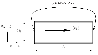
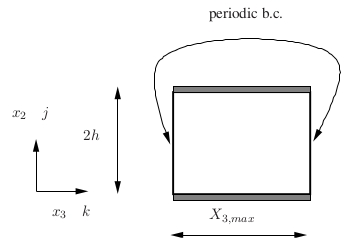
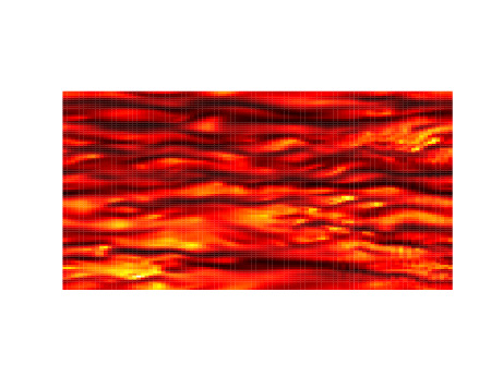
Instantaneous w' fluctuations at y+=9
- k-omega DES of the hill flow. Periodic boundary conditions in streamwise and
spanwise directions.
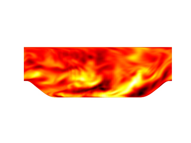
Instantaneous spanwise fluctuation
- k-omega DES of the channel flow at Reτ = 5200.
Periodic boundary conditions in streamwise and
spanwise directions.
Resolved (blue) and modeled (red) shear stresses compared with DNS (markers)
- Channel flow with inlet-outlet Reτ = 395. Periodic boundary conditions in
spanwise direction.
Predicted friction velocity vs. x. Target value is one
Shear stresses compared with DNS (markers)
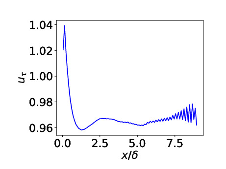
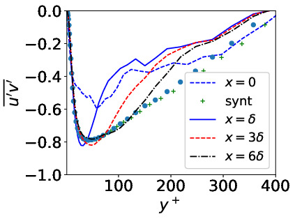
- Channel flowwith inlet-outlet Reτ = 5200. Periodic boundary conditions in
spanwise direction.
Predicted friction velocity vs. x. Target value is one

Shear stresses compared with fully developed DES and inlet synthetic fluctuations (markers)
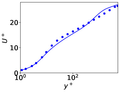
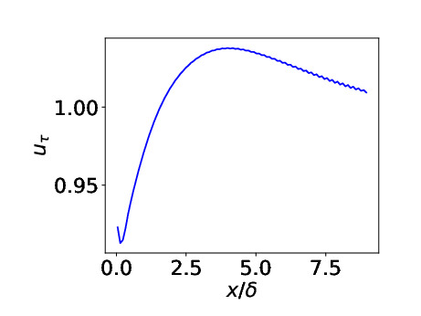
- Flat-plate boundary layer. Δx+=40, Δz+=104. LES (Reθ,inlet;=2 400)
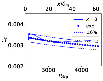
Predicted skin friction vs. Reθ. Markers: expts
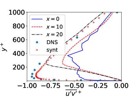
Shear stresses compared with DNS and inlet synthetic fluctuations (markers)
- Hump flow, Re=9.36E+5)
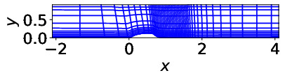
The grid (every 8th grid line is shown)
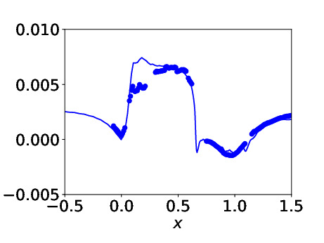
Predicted skin friction. Markers: expts
- Couette-Poiseuille flow, DNS (ReΔU2h=40000)
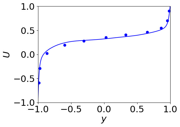
Velocity
pyCALC-LES currently includes two zero-equation SGS models (Smagorinsky and WALE) and two two-equation models (the PANS
model and the k-omega DES model).
Workshops
The course includes eight workshops (two hours every second week)
during which the PhD students be supervised how to implement different turbulence models
and synthetic inlet/emmbedded fluctuations in the pyCALC-LES.
In the workshops, the participants will use pyCALC-LES.
installed on their lap-top or on their desktop.
The following Python packages are used
- python 3.8
- from scipy import sparse
- import numpy as np
- import pyamg
- On Ubuntu I installed it with the command 'conda install -c anaconda pyamg'
- from scipy.sparse import spdiags,linalg
In the workshops, the student will be guided to carry out fast RANS and DES simulations (30-60 minutes)
of the flow in a boundary layer and half a channel.
- Part I of the workshop is described in
Section Workshop in pyCALC-LES:
- Part II of the workshop is described
here
In Part II, Students could also choose to make a numerical task. In 2021, the Phd students
did these project:
- Algebraic Multigrid methods on the GPU to
accelerate pyCALC-LES
- Implementation of a hybrid RANS-LES
approach using temporal filtering
- Implementation of energy equation and laminar natural
convection on pyCALC-solver
- Implementation of the dynamic SGS
model in pyCALC-LES
- Comparative assessment of the Synthetic Eddy Method
and the Synthetic Turbulence Generator in boundary
layer flow using pyCalc
Suggestions on projects this year (2023) could be
- Parallelize pyCALC-LES on many cores (but within one node, i.e. common memory)
- Re-write the time-consuming parts of pyCALC-LES to Numba or PyCu so that
the execution takes place on the GPU (the sparse-matrix
solver already run on the CPU). This should probably be limimted to DNS or LES (with the SGS model
WALE, for example)
- Implement a new physical model (turbulence, transition, boiling, multiphase, ...)
The examination consists of presenting the work in front of the class as well as in a report.
Department of Mechanics and Maritime Sciences
Division of Fluid Dynamice
|